Plotting pre-post results in R
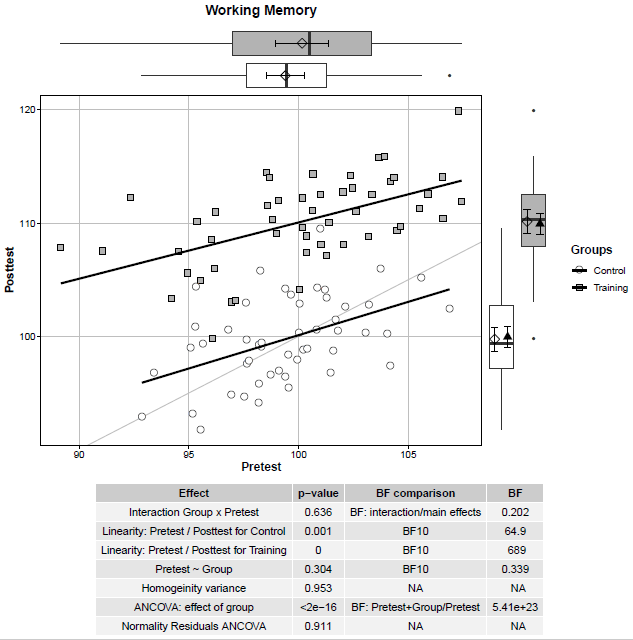
A quick code to create a useful plot to visualise pre- and post-test results. I was inspired by this post, this post, and this post. A scatterplot between pre-test and post-test scores for the control and the training group is presented. The straight black lines represent correlations between pre-test and post-test scores within the two groups. The straight lightgrey line represents the same values at pre-test and post-test –> Subjects above the line display a better performance at post-test compared to pre-test. At the margins, the boxplots are reported as well as the mean (i.e., diamond) and 95% confidence intervals (i.e., error bars). In the case of the post-test scores (plot on the right margin), the adjusted means (i.e., black triangles) and associated 95% confidence intervals (i.e., error bars) are reported. The table reports the results for the ANCOVA and its assumptions. In this example, participants in the training group show an improvement in a Working Memory task.
# Seed
set.seed(42)

# Packages
library(ggplot2)
library(Hmisc)
library(cowplot)
library(mvtnorm)
library(reshape2)
library(ggpubr)
library(ggExtra)
library(gridExtra)
library(car)
library(apaTables)
library(BayesFactor)
library(dplyr)
library(effects)


# Generate some correlated values
Scores <- c(rmvnorm(n=100,mean=c(100,100),sigma=matrix(c(15,0.8*sqrt(100),
0.8*sqrt(100),15),2,2)))

# Add improvement for the training group
improvement <- c(rep(0,100), rep(10, 50), rep(0,50))
Scores <- Scores + improvement

# Groups
Groups <- rep(rep(c("Training", "Control"), each=50),2)

# Session
Session <- rep(c("Pretest", "Posttest"), each = 100)

# Subject ID
Subject <- as.factor(rep(1:100,2))

# Long format
df_long <- data.frame(Subject, Session, Groups, Scores)

# Wide format
df_wide <-  dcast(df_long, Subject + Groups ~ Session, value.var="Scores")

# ANCOVA

# set orthogonal contrasts
contrasts(df_wide$Groups)=contr.poly(length(unique(df_wide$Groups)))

# Assumption 1: equality of slopes–interaction is not significiant.
res_int <- aov(Posttest ~ Pretest + Groups + Groups:Pretest, data = df_wide)
pvalue_int <- summary(res_int)[[1]][["Pr(>F)"]][3]
res_int_bf <- lmBF(Posttest ~ Pretest + Groups + Groups:Pretest, data = df_wide, whichRandom = "Subject")
res_maineff_bf <- lmBF(Posttest ~ Pretest + Groups, data = df_wide, whichRandom = "Subject")
bf_int <- extractBF(res_int_bf/res_maineff_bf, onlybf = T)

# Assumption 2: linearity of slopes
gp <- group_by(df_wide, Groups)
cor_pvalues <- as.data.frame(dplyr::summarize(gp, cor.test(Pretest, Posttest)$p.value))
names(cor_pvalues)[2] <- "pval"
cor_bf <- as.data.frame(dplyr::summarize(gp, extractBF(correlationBF(y = Pretest, x = Posttest), onlybf = T)))
names(cor_bf)[2] <- "bf"

# Assumption 3: Equality of the groups on the covariate
res_comp_cov <- aov(Pretest ~ Groups, data = df_wide)
pvalue_comp_cov <- summary(res_comp_cov)[[1]][["Pr(>F)"]][1]
res_comp_cov_bf <- anovaBF(Pretest ~ Groups, data = df_wide, whichRandom = "Subject")
bf_comp_cov <- extractBF(res_comp_cov_bf, onlybf = T)

# Assumption 4: Homogeneity of variance
res_omvar <- leveneTest(Posttest ~ Groups, center = median, data = df_wide)
pvalue_omvar <- res_omvar$`Pr(>F)`[1]

# Results ANCOVA
res_anc <- aov(Posttest ~ Pretest + Groups, data = df_wide)
res_anc_an <- Anova(res_anc, type=3)
pvalue_anc <- res_anc_an$`Pr(>F)`[3]
res_anc_bf <- lmBF(Posttest ~ Pretest + Groups, data = df_wide, whichRandom = "Subject")
res_effcov_bf <- lmBF(Posttest ~ Pretest, data = df_wide, whichRandom = "Subject")
bf_anc <- extractBF(res_anc_bf/res_effcov_bf, onlybf = T)
pvalue_shap_anc <- shapiro.test(resid(res_anc))$p.value

# Adjusted means
adj_means <- as.data.frame(effect("Groups", res_anc))

# Table with results
result_text <- c("Interaction Group x Pretest",
                 paste("Linearity: Pretest / Posttest for", cor_pvalues$Groups[1]),
                 paste("Linearity: Pretest / Posttest for", cor_pvalues$Groups[2]),
                 "Pretest ~ Group",
                 "Homogeinity variance",
                 "ANCOVA: effect of group",
                 "Normality Residuals ANCOVA")

p_values <- c(pvalue_int,
              cor_pvalues$pval[1],
              cor_pvalues$pval[2],
              pvalue_comp_cov,
              pvalue_omvar,
              pvalue_anc,
              pvalue_shap_anc)

bfs_text <- c("BF: interaction/main effects",
              "BF10",
              "BF10",
              "BF10",
              NA,
              "BF: Pretest+Group/Pretest",
              NA)

bfs <- c(bf_int,
         cor_bf$bf[1],
         cor_bf$bf[2],
         bf_comp_cov,
         NA,
         bf_anc,
         NA)

table_res <- data.frame(result_text, format.pval(p_values, digits = 3), bfs_text, formatC(bfs, digits = 3))
row.names(table_res)<-NULL
names(table_res) <- c("Effect", "p-value", "BF comparison", "BF")
tab_res <- ggtexttable(table_res, rows=NULL)

# Main scatterplot
pmain <- ggplot(data = df_wide, aes(x=Pretest, y=Posttest, shape=Groups, fill=Groups)) +
  geom_abline(slope = 1, col="grey") +
  geom_point(size = 3) +
  scale_shape_manual(values = c(21,22)) +
  scale_fill_manual(values = c("white", "grey70")) +
  stat_smooth(method = "lm", se = F, col="Black") +
  theme_classic(base_size = 12) +
  theme(axis.title.x = element_text(face="bold"),
        axis.title.y = element_text(face="bold"),
        legend.title = element_text(face="bold"),
        strip.text = element_text(face="bold"),
        axis.text.x = element_text(colour = "Black"),
        axis.text.y = element_text(colour = "Black"),
        axis.ticks.x = element_line(colour = "Black", size = 0.2),
        axis.ticks.y = element_line(colour = "Black", size = 0.2),
        axis.line.x = element_line(size = 0.2),
        axis.line.y = element_line(size = 0.2),
        strip.background = element_rect(size = 0.2),
        panel.border = element_rect(size = 0.2,color="black", fill=NA),
        plot.title = element_text(face="bold", hjust = 0.5),
        legend.position="right",
        panel.grid.major = element_line(size = (0.1), colour="grey"),
        panel.grid.minor = element_blank()) +
  ggtitle("Working Memory")

# Boxplot for pre-test
xbox <- axis_canvas(pmain, axis = "x", coord_flip = TRUE) +
  geom_boxplot(data = df_wide, aes(y = Pretest, x = Groups, fill=Groups), outlier.size = 1) +
  stat_summary(data = df_wide, aes(y = Pretest, x = Groups), fun.data = "mean_cl_normal",colour="black",geom="errorbar", size=0.5, width=0.2) +
  stat_summary(data = df_wide, aes(y = Pretest, x = Groups), fun.y ="mean", geom="point", shape=5, size=3) +
  scale_x_discrete() +
  coord_flip() +
  scale_fill_manual(values = c("white", "grey70"))

# Boxplot for post-test
pd=0.2
ybox <- axis_canvas(pmain, axis = "y") +
  geom_boxplot(data = df_wide, aes(y = Posttest, x = Groups, fill=Groups), outlier.size = 1) +
  stat_summary(data = df_wide, aes(y = Posttest, x = Groups),
               fun.data = "mean_cl_normal",colour="black",geom="errorbar", size=0.5, width=0.2, positio=position_nudge(x = -pd)) +
  stat_summary(data = df_wide, aes(y = Posttest, x = Groups), fun.y ="mean", geom="point", shape=5, size=3, positio=position_nudge(x = -pd)) +
  scale_x_discrete() +
  scale_fill_manual(values = c("white", "grey70")) +
  geom_point(data = adj_means, aes(y = fit, x = Groups), color = "Black", size = 3, shape=17, position = position_nudge(pd)) +
  geom_errorbar(data = adj_means, aes(y = fit, ymin = lower, ymax=upper, x = Groups), size=0.5, width=0.2, position = position_nudge(pd))

# Combine plots
p1 <- insert_xaxis_grob(pmain, xbox, grid::unit(1, "in"), position = "top")
p2 <- insert_yaxis_grob(p1, ybox, grid::unit(1, "in"), position = "right")
# Show the plot
ggarrange(p2, tab_res, nrow=2, heights = c(3,1))


Comments
Post a Comment